Functions are a core concept in the study of calculus. In this section we outline common representations of functions and some general properties that we will use throughout future sections.
Subsection1.2.1Functions and their Representations
Understanding systems is all about being able to describe the relationship between the quantities involved. The population of a species is related to time, the energy an animal exerts when running is related to its speed, and the growth of a plant is related to its exposure to sunlight. Equations, tables, and graphs are all mathematical objects that help us represent relationships between quantities, and it is beneficial to be able to represent a single relationship in multiple different ways.
Given two related quantities \(x\) and \(y\text{,}\) we say \(y\) is a function of \(x\) if every \(x\) value in the relationship is related to exactly one \(y\) value.
Using this terminology with our previous illustrations, we would say a population is a function of time, energy is a function of speed, and the height of a plant is a function of sunlight exposure. Notice that there is an ordering implied when we talk about function relationships. When we say “\(y\) is a function of \(x\)”, we call \(x\) the input (or independent variable) and \(y\) the output (or dependent variable).
In \(y = x+1\text{,}\)\(y\) is a function of \(x\text{.}\) Our reasoning will sound different depending on whether you are looking at the equation, table, or graph, but in all cases our reasoning is based on Definition 1.2.1:
Warning: When relationships are represented via tables, it is possible you have limited information about the relationship. Unless you are told that the table shows every \(x,y\) pair in the relationship, you should assume there may be other \(x,y\) pairs in the relationship not listed in the table.
Graph: If you pick an \(x\) value and draw a vertical line at that \(x\) value, you will intersect the graph exactly once. This means each \(x\) value corresponds to exactly one \(y\) value. This is known as the vertical line test to determine if the graph of a relationship represents a function relationship.
In \(y^2 = x+1\text{,}\)\(y\) is not a function of \(x\text{.}\) Our reasoning will sound different depending on whether you are looking at the equation, table, or graph, but in all cases our reasoning is based on Definition 1.2.1:
Equation: For an \(x\) value, the corresponding \(y\) value is obtained by the rule \(\pm \sqrt{x+1}\text{.}\) This means that when \(x=0\text{,}\) for example, the associated \(y\) values are \(\pm 1\text{.}\) This means there is an \(x\) value associated to more than one \(y\) value, and so this relationship is not a function.
Table: There are \(x\) values in the table listed more than once, and associated with different \(y\) values. This means there are \(x\) values in the relationship associated with more than one \(y\) value.
Graph: You can pick an \(x\) value and draw a vertical line at that \(x\) value such that you intersect the graph more than once. This means you have found an \(x\) value which corresponds to more than one \(y\) value. This is known as the vertical line test to determine if the graph of a relationship represents a function relationship.
Practice using Definition 1.2.1 by answering each question below. Focus on verbalizing your thought process. Your reasoning is more important than your final answer.
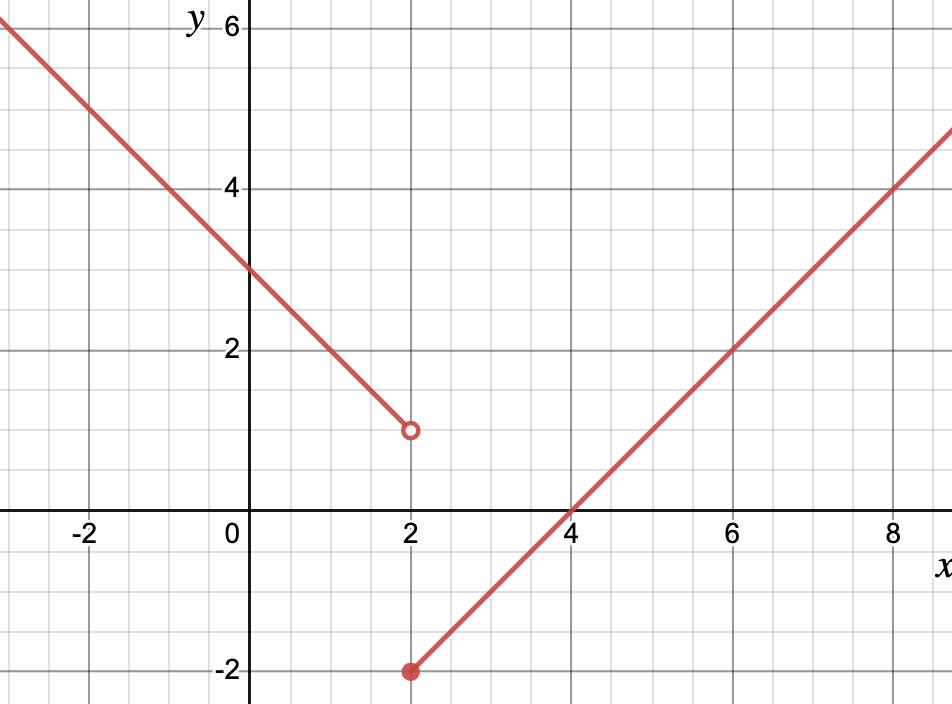
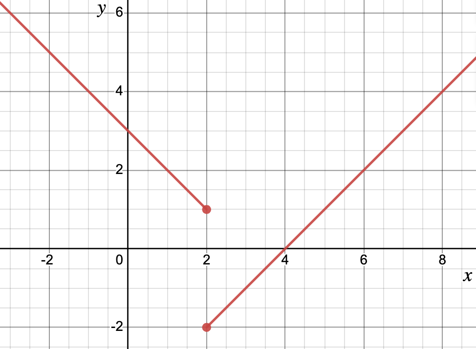
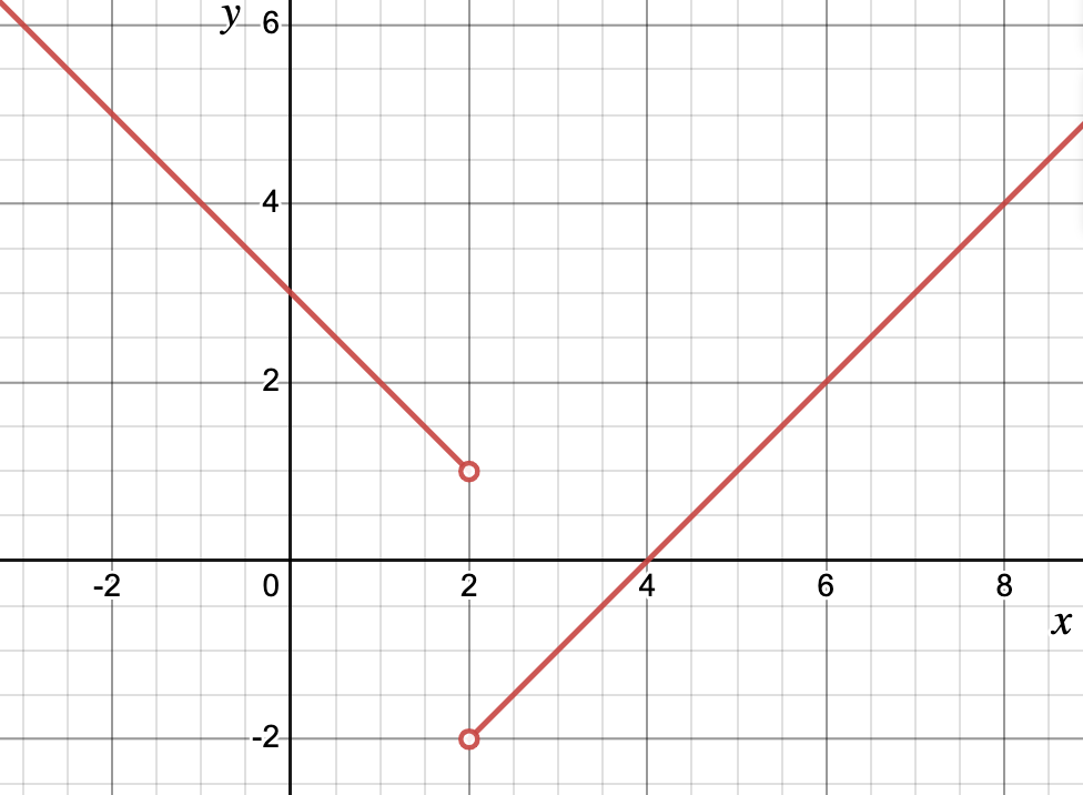
A decreasing line ending with a closed circle at x equal 2 and y equal 1. An increasing line starting with a closed circle at x equal 2 and y equal -2.
The graphs in Activity 1.2.2 are very similar, but they all represent different relationships. Of those that are functions, they differ in their domain and range, which we define below:
The domain of a function is typically determined by one or more of the following:
Operations: There may be operations used to define a function which are undefined for specific inputs. For example, in \(y=\frac{1}{x}\text{,}\)\(x=0\) is not in the domain because the operation of division by \(0\) is not defined.
Context: When a function is used as a model, there may be some input values that don’t make sense for what the function represents. For example, if height is a function of time given by \(h = t^2\text{,}\) negative \(t\) values are not in the domain even though operationally the function is defined for negative \(t\) values.
When given a function relationship, there are two main ways we might express that relationship:
Explicit Function: An explicit function describes the output (or dependent variable) explicitly in terms of the input (or independent variable). For example, \(y=x+1\) is an explicit function. However, moving forward we will most often write explicit functions using function notation, which means we write the output (dependent variable) as \(f(x)\) instead of \(y\text{.}\) The function \(y=x+1\) is written using function notation as \(f(x) = x+1\text{.}\) Note that we may name the function whatever we’d like (it does not have to be “\(f\)”). For example, if the output was “population” and the input was “time”, we might call our function \(p(t)\text{.}\)
Recursive Function: A recursive function is typically used when modeling discrete systems, and describes the next output (or dependent variable) in terms of the current output (or dependent variable). For example, \(p_{t+1} = p_t +2 \) is a recursive function. In words, this function says “the next output is equal to the current output plus two.” Notice that this relationship does have an independent variable \(t\text{,}\) it is just not used in describing the relationship like in an explicit function.
As illustrated in Exercise 1.1.4.2, modeling real systems typically involves representing quantities with letters and numbers. It is important that we know how to interpret the letters that we see in function representations.
The function \(h(t)=mt+b\) describes a relationship whose graph looks like a straight line. One benefit of using function notation is that it clearly indicates to us which letters represent variables. The notation “\(h(t)\)” tells us that \(t\) is the input (or independent variable), and \(h(t)\) is the output (or dependent variable). This means that for a fixed line, the input value \(t\) can change, and \(h(t)\) changes along with it.
Once we identify the independent and dependent variable, every other letter represents a parameter. In this example, \(m\) and \(b\) are parameters. This means that for a fixed line, \(m\) and \(b\) are constant values.
One benefit of using parameters is that it allows us to describe many models at once, and we can then analyze how a specific system behaves based on its parameter values.
Just as there are ways to combine two numbers to get a new number, we can also combine two functions to get a new function. Given two functions \(g(x)\) and \(k(x)\text{,}\) we can define the following combinations:
Let \(m(w)\) be the number of mosquitos entering a house if \(w\) windows are open, and \(b(m)\) be the number of mosquito bites someone gets if there are \(m\) mosquitos in a house.
We noticed in Definition 1.2.1 that there is an order implied in a function relationship. Depending on the question you would like to answer, the ordering of the function may or may not be desirable. For example, if you had a model where population was a function of time, and you wanted to know when the population would reach \(1,000\text{,}\) this ordering would be desirable. However, if the population was decreasing and you wanted to know after how many years the population would become extinct, it may be desirable to have a model expressing time as a function of population. The property of being able to switch input and output and still have a function relationship is what we define below:
Let \(f(x)=y\) be a function of \(x\text{.}\) If \(x\) is also a function of \(y\text{,}\) we say that \(f\) is invertible. We denote \(x\) as a function of \(y\) as \(f^{-1}\text{,}\) and call it the inverse function of \(f\).
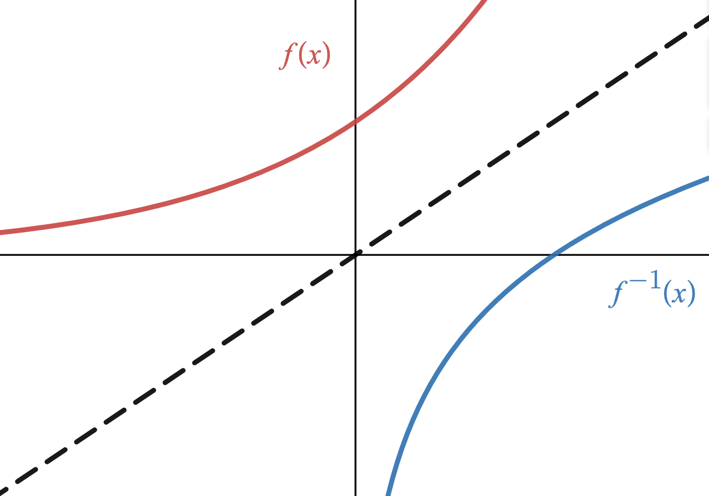
To determine if this function has an inverse function, we must determine if the relationship obtained by swapping input and output is also a function. We can test this directly on the graph of \(f\) by remembering the vertical line test used in Example 1.2.2, and thinking about how vertical lines change when we swap input and output.
A vertical line in the \(x,y\) plane is a line whose points have a constant \(x\) value. For example, the points \((1,0), (1,1), (1,2), (1,3)\) all lie on the vertical line \(x=1\text{.}\) When we swap input and output, those points become \((0,1), (1,1), (2,1), (3,1)\) , which all lie on the horizontal line \(y=1\text{.}\) So we can determine if the function \(f\) is invertible by drawing horizontal lines on the graph of \(f\text{.}\) If every horizontal line intersects the graph at most once, then \(f\) is invertible. Otherwise, the function \(f\) is not invertible.
This is known as the horizontal line test for testing invertibility. In this example we see the function is invertible, and we can visualize the graph of \(f^{-1}\) by reflecting the graph of \(f\) over the diagonal line \(y=x\text{:}\)
Let \(f(x)= 3x + 1\text{.}\) If \(f\) has an inverse function, \(x\) would be the output and \(f(x)\) would be the input. As an equation, this means we will try to re-write the function relationship as “\(x=\)”. For notational purposes, before we start the computation we’ll write the function as \(y=3x+1\) instead of using function notation.
\begin{align*}
y \amp=3x+1\\
y-1 \amp= 3x\\
\dfrac{y-1}{3}\amp= x\\
x \amp= \dfrac{y-1}{3}
\end{align*}
This shows us that \(f\) is invertible, and also what the rule is for the inverse function. Instead of using \(x\) as the output variable, we switch back to the standard notation and write \(f^{-1}\) as a function of \(x\text{:}\)\(f(x)=3x+1\) and \(f^{-1}(x) = \dfrac{x-1}{3}\text{.}\)
Invertible functions and their inverse functions have a special property under composition. As illustrated in Example 1.2.8, the order of composition matters. That is, for two functions \(f(x)\) and \(g(x)\text{,}\) the compositions \(f(g(x))\) and \(g(f(x))\) are, in general, different. However, composition with an invertible function and its inverse function is an example of a special case when the order does not matter. Even more, the composition will always result in the same function:
We mentioned in Section 1.1 that a main goal in mathematical modeling is to study how systems change. Given a function, one way we can describe how the function changes over time is by computing an average rate of change. This is also a foundational concept that will be used to extend our tools for describing change in Chapter 2.
Being able to compute an average rate of change is necessary, but understanding what an average rate of change represents graphically will be even more important for our future developments in describing how functions change. Use the interactive provided to complete the statements below before viewing the answers.
Graphically, the value of \(AROC_{[a,b]}\) describes Answer.
whether the line connecting the two points \((a,f(a))\) and \((b,f(b))\) increases, decreases, or stays the same. Further, the larger the average rate of change is in absolute value, the steeper the line will increase or decrease. The line connecting the two points is called the secant line.
A letter in function may represent a variable (a changing quantity) or a parameter ( a constant quantity). Function notation is useful for helping us recognize the variables in a model.
We can combine functions like numbers using addition, subtraction, multiplication, and division. We can also put functions inside of other functions using composition.
We can describe how a function changes over a specific time interval by computing the average rate of change over that time interval. Graphically, this number tells us the steepness of the secant line connecting the two end points, and if the secant line is increasing or decreasing.
Give an example of a relationship in which \(y\) is not a function of \(x\text{.}\) Write a sentence explaining why your example works, and represent your example as an equation, table, and graph.
Give an example of a relationship in which \(y\) is a function of \(x\) but is not an invertible function. Write a sentence explaining why your example works, and represent your example as an equation, table, and graph.
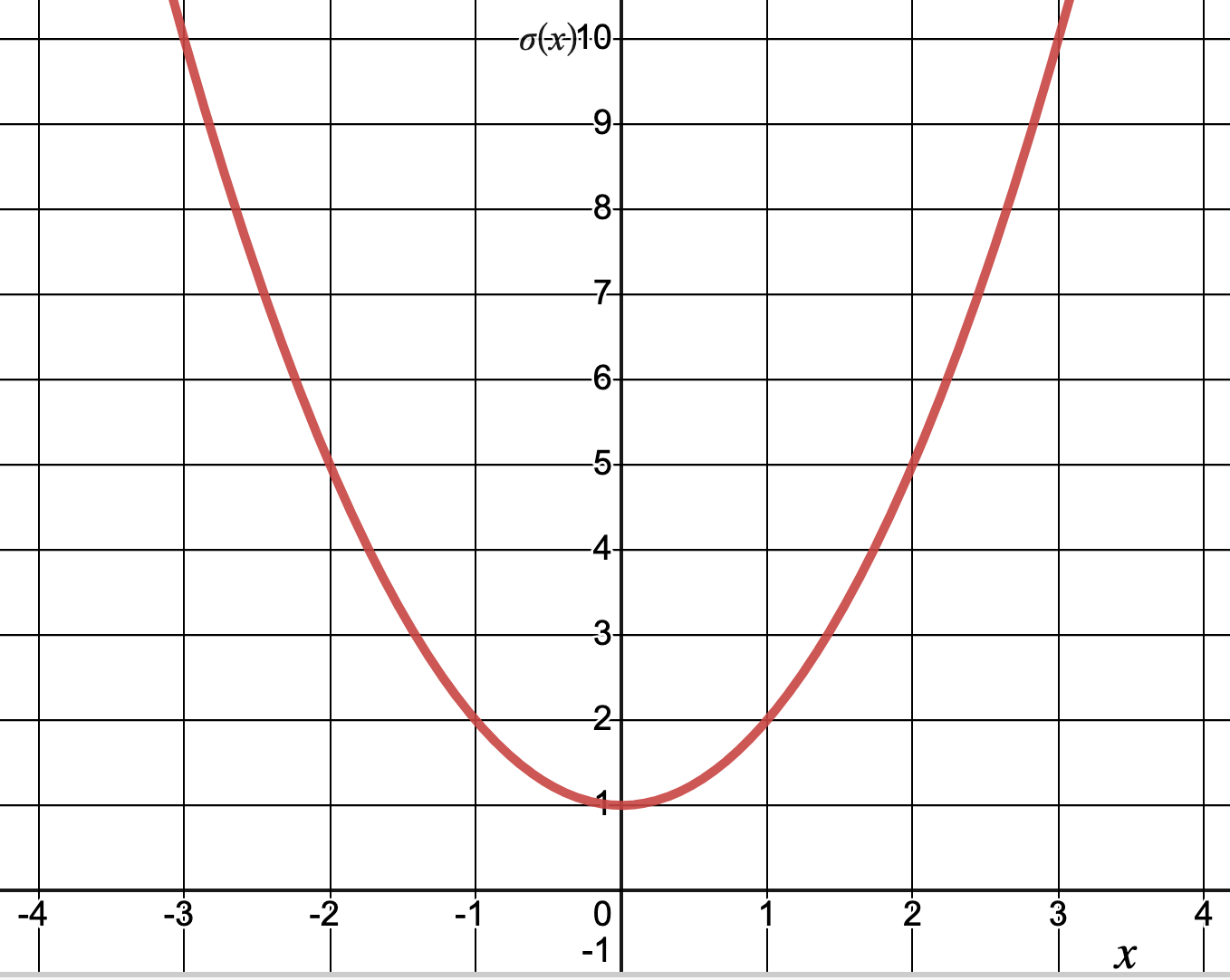
Let \(\sigma(x) = x^2 +1\text{.}\) Calculate each average rate of change below. Then use the graph provided to illustrate what each calculation represents graphically.