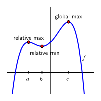
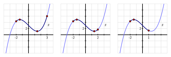
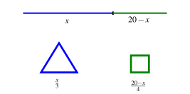
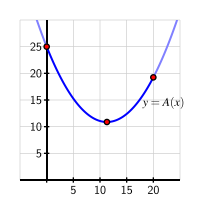
Example 3.5.8 and
Activity 3.5.11 illustrate standard steps that we undertake in almost every applied optimization problem: we draw a picture to demonstrate the situation, introduce one or more variables to represent quantities that are changing, find a function that models the quantity to be optimized, and then decide on an appropriate domain for that function. Once that is done, we are in the familiar situation of finding the absolute minimum and maximum of a function over a particular domain, so we apply the calculus ideas that we have been studying in this section.
We complete this section with a final optimization application relevant to foraging individuals in a system where food is obtained in discrete spaces which require time to travel between. One example is a bee traveling between flowers for nectar. If the bee’s goal is to maximize its average food collection rate per flower, it must decide whether to stay on the current flower, where its rate of food collection is decreasing as the nectar is depleted, or travel to another flower with more nectar, but lose the time it takes to travel there.
To find the optimal amount of time the bee should stay on each flower, we must determine a model for the quantity we’d like to maximize, the bee’s average food collection rate per flower after \(t\) seconds, which we will call \(r(t)\text{.}\) This includes the non-zero travel time it takes to get to another flower, which we will call \(\tau\text{.}\) Assume \(f(t)\) is the amount of food collected after \(t\) seconds on a flower, and that \(f(t)\) is continuous and satisfies \(f''(t) \lt 0 \text{.}\) This last assumption means \(f\) is concave down, or that the bee’s food collection rate on the flower decreases as time goes on and nectar is depleted. We can then write \(r(t)\) as
\begin{equation*}
r(t) = \dfrac{\text{food collected after }t \text{ seconds on flower}}{\text{total time before next flower}} = \dfrac{f(t)}{t + \tau}\text{.}
\end{equation*}
The domain of \(r(t)\) is the interval \([0,\infty)\text{.}\) To find the maximum value of \(r\) on this domain we first search for critical numbers of \(r\) in \([0,\infty)\text{.}\) We compute the first derivative of \(r\) as
\begin{equation*}
r'(t) = \dfrac{f'(t)(t+\tau) - f(t) \cdot 1}{(t+\tau)^2}
\end{equation*}
Note that the denominator is always positive, so \(r'(t)\) is not undefined in the domain \([0,\infty)\text{.}\) Thus, \(t_c\) is a critical number if \(r'(t_c)=0\text{,}\) which is true when \(f'(t_c)(t_c+\tau) - f(t_c) =0\text{.}\) This is equivalent to \(f'(t_c)(t_c+\tau) = f(t_c)\text{,}\) which is equivalent to
\begin{equation*}
f'(t_c) = \dfrac{f(t_c)}{t_c+\tau} = r(t_c)\text{.}
\end{equation*}
In words, this says that if a time \(t_c\) is a critical number, then the instantaneous rate of change of the bee’s food collection on the flower at time \(t_c\) is the same as the bee’s average collection rate over the \((t_c + \tau)\) seconds it takes to be on the next flower. To verify that a maximum value occurs at a critical number \(t_c\text{,}\) the assumption that \(f''(t) \lt 0\) is important. It is a good exercise in computing derivatives to verify that if we compute \(r''(t)\text{,}\) evaluate \(r''(t_c)\) and then simplify, we get
\begin{equation*}
r''(t_c) = \dfrac{f''(t_c)}{t_c + \tau}\text{.}
\end{equation*}
Since
\(t_c + \tau \gt 0\) and under the assumption that
\(f''(t_c) \lt 0\text{,}\) this means that
\(r''(t_c) \lt 0\text{.}\) Hence, by the second derivative test, a local maximum of
\(r(t)\) occurs at the critical number
\(t_c\text{.}\) Further, every critical number
\(t_c\) in the domain
\([0,\infty)\) satisfies this property, and so every critical number in
\([0,\infty)\) is a local maximum. Since
\(r(t)\) is a continuous function on the domain
\([0,\infty)\text{,}\) there can only be one such critical point. By
Fact 3.5.3, a global maximum of
\(r(t)\) also occurs at the critical number
\(t_c\text{.}\)